Introduction
Thermal systems are difficult to model because of the complexity of the modes of heat transfer: conduction, convection, and radiation. Thermal conductivity can vary depending on the temperature and direction (such as with some crystals). Convection needs to consider fluid dynamics, which can be free or forced, laminar or turbulent. Thermal radiation is electromagnetic radiation, and as such, can be reflected or refracted. Through finite element methods it is possible to model all the modes of heat transfer, but this tends to be computational expensive.
Here I will show how to empirically measure a simple thermal system and fit a simple thermal model to estimate the thermal capacity and rate of heat loss of the system.
Setup
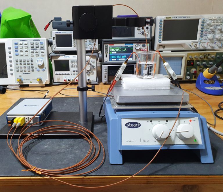
A 35.37 g borosilicate glass beaker was filled with 40.00 g of mineral oil and a small magnetic bar was added to stir the liquid with a magnetic stirrer. A tiny piece of nichrome wire was submerged into the liquid to heat it with an SMU connected to the cable through a 4-wire connection. Two thermocouples were used, one to measure the temperature of the liquid, and the other to measure the ambient temperature. The beaker was kept thermally insulated from the magnetic stirrer so that the hot plate would not act as a heatsink and make the modelling of the system more complex.
Probing Protocol
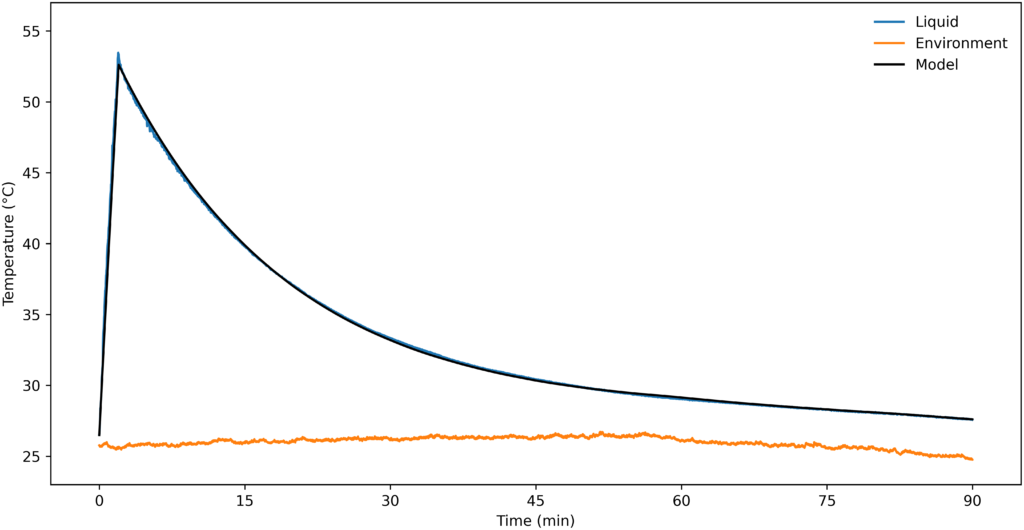
The system behavior was probed by making continuous temperature measurement of the two thermocouples while injecting ~22 W (4 V constant voltage) of heat for 120 s into the liquid through the nichrome wire. The temperature was measured for 90 min and the magnetic stirrer was left running during the whole process to keep the temperature uniform.
The temperature time series looked like this:
One interesting thing that I noticed is that the initial temperature of the liquid did not match the environment temperature. Some factors that may have caused this mismatch are the slow liquid temperature adaption to the ambient temperature, thermocouple differences and the heat injected through the rotating magnetic bar.
Thermal Model #1
To model the temperature behavior I initially used the following ordinary differential equation (ODE):
\begin{align*}
\frac{dT(t)}{dt} = \frac{p(t) + G(T_e(t)-T(t))}{C}
\end{align*}
Where:
\(T\) is the temperature of the beaker in °C.
\(p\) is the rate of heat injected into the filled-beaker through the nichrome wire in W.
\(G\) is the thermal conductance between the filled-beaker and the environment in W/°C.
\(Te\) is the environment temperature in °C.
\(C\) is the thermal capacity of the filled-beaker in J/°C.
I optimized the C and G values to find the best fit (minimum sum of squared residuals) to the measured data. For a \(C\) of 102.7 J/°C, and a \(G\) of 0.072 W/°C I got a root mean square residual (RMSR) of 0.734 °C.
The fit was not bad, but not great either, so I decided to try to improve the model.
Thermal Model #2
To eliminate the effect of the temperature offset I added a \(To\) parameter to model.
\begin{align*}
\frac{dT(t)}{dt} = \frac{p(t) + G(T_e(t)+T_o-T(t))}{C}
\end{align*}
This time for a \(C\) of 96.1 J/°C, a \(G\) of 0.088 W/°C and a \(T_o\) of 1.8 °C I was able to get an RMSR of 0.235 °C.
To check how close my estimation of the thermal capacity was, I compared it to what it should be for 35.37 g of borosilicate glass and 40.00 g of mineral oil. I found on the literature that the specific thermal capacity of borosilicate and mineral oil are 0.83 J/(g °C) and 1.67 J/(g °C) respectively. So the thermal capacity of the beaker filled with oil (without considering the magnetic bar and wire) should be: 35.37 * 0.83 + 40 * 1.67 = 96.2 J/°C. The surprisingly close match between the estimated and and the “true” thermal capacity was far better than what I expected, and was probably the result of many errors cancelling each other out.
Conclusion
In this experiment I showed how I was able to empirically estimate the thermal capacity and conductivity of a system. I showed that even though thermal systems can get extremely complex to simulate, in some cases it is possible to achieve accurate results through the usage of simple thermal models that take into consideration only the dominating thermal effects.


